
A tabletop soccer serves as a showcase for demonstrating the capabilities of SAP Data Intelligence, SAP Warehouse Cloud and SAP Analytics Cloud. The article gives an overview on the setup.
The CAMELOT Village was the global event celebrating the company’s 25 years. More than 600 colleagues have participated in Mayrhofen and worked in different activities and workshops.
One of the main attractions among these activities was the marketplace where the company’s divisions presented showcases on current topics from customer projects as well as from internal projects.
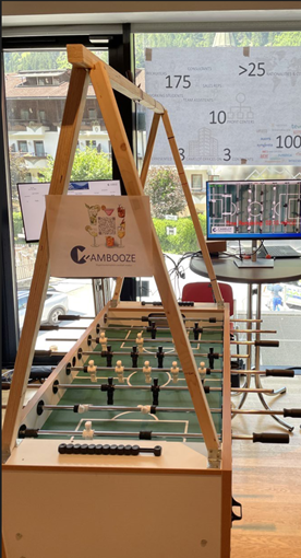
For this occasion, some data experts built a tabletop soccer game demonstrating the capabilities of different SAP technologies such as SAP Data Intelligence, SAP Warehouse Cloud and SAP Analytics Cloud to count the statistics of the game in real-time and then to show it on an SAC dashboard.
The soccer table was extended within a frame that hold a camera on top. The camera height was adjusted manually at first to cover the whole playing field. The camera was then mounted on the soccer table with a wooden extended frame to placed it firmly in such a way that it can provide the continuous real time data to process it and to make sure that the camera will not be disturbed during the game.
The article gives an overview on the data flow architecture and the underlying python application.
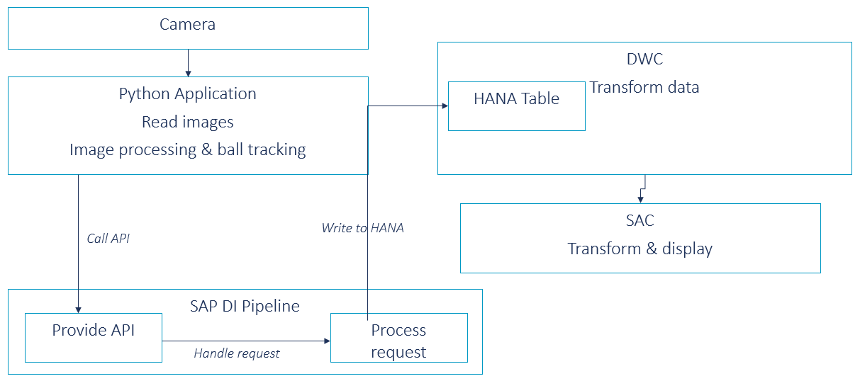
Overview of the Data Flow Architecture
Figure 2 gives an overview of the overall data flow architecture. On the local side, a Python application handles the data processing. It streams and captures data from the camera mounted on top of the kicker table and processes the data to extract several events happening on the field.
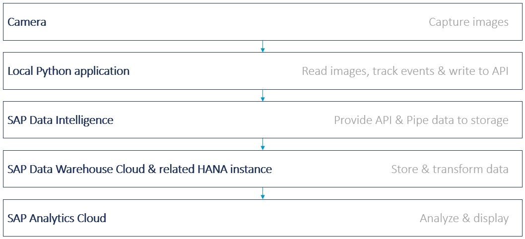
These events are then communicated to a REST API which is provided by SAP Data Intelligence. The REST API is implemented as a pipeline in SAP Data Intelligence which handles the data on every request. This means it stores and retrieves information from/to a HANA database, which in this case was the underlying HANA database of the SAP Data Warehouse Cloud. SAP Data Warehouse Cloud itself then extracts the data in views and provides it to SAP Analytics Cloud which, finally, analyzes the data it retrieves and displays it on a dashboard.
Data Recording
The different camera models which were tested as well as the final camera model implemented for the project are listed as follows.
- Model 1 with high framerate was not adopted as API communication did not work flawlessly.
- Model 2 with 60fps did not work out as the provided image had a strange color.
- Model 3 with 30fps was finally used, but is not optimal, as its frame rate is too low to take high speed shots.
If you want to test for a camera for your setup, we would advise to look for cameras with more than 30fps – and you might need to test several models.
Local Python Application
The ball tracking was performed in a local Python module based on OpenCV, which is a widely used open-source library for computer vision. In addition to image processing, OpenCV also supports the processing of videos, both recorded and live. With OpenCV, we can programmatically open capturing devices like webcams, and thereafter feed each captured frame to our downstream ball tracking function. This makes it a perfect fit for our use case.
Initial Image Processing
The number of frames which are returned by OpenCV depends on the camera’s frame rate. In the underlying use case, the frame rate is 30 frames per second. Every frame is returned as an image array by OpenCV. Before we send this image to the ball tracking functionality, we pass it through some processing steps, which are:
- resizing the image,
- cropping the image so that only the actual field remains,
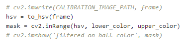
- converting it to the HSV color space, as this is the best suited color space for object detection,
- creating an image mask to identify only the pixels that are within the color range set in the ball calibration step,
- apply dilation and morphology extraction on the remaining pixels,
- find the contours within the dilated and morphed image.
After this cascade of processing steps, the contours found in the image are passed to the actual ball tracking function.
Calibration for ball detection
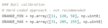
The ball is tracked by finding the pixels on the image that are 1) within a similar color range as the color of the ball and 2) together form a circle that resembles the shape of the ball that is used for playing. Hence, we need to set appropriate thresholds for the radius of a detected circle to recognize it as the actual ball. By setting these thresholds we also filter out noise, e.g., from light reflections.
To set the color range of the ball, we use an initial calibration step every time the ball tracking module is started from new. For the calibration step to work, the ball must reside at the field’s center point when starting the module, since the center pixel of the image is taken as the anchor for defining the color range. We expand the color range around the center pixel by adding/subtracting some tolerance as the HSV values might slightly vary due to light reflections and shadows.
Ball tracking
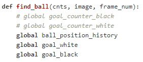
The ball tracking function works with the contours of the processed image. Contours are a very useful tool for shape analysis and object detection. In our use case, they allow us to identify shapes that resemble the ball. For each contour, we identify the circumference and radius of its minimum enclosing circle, and only if both values are within our defined thresholds, they are considered as ball candidates. The thresholds were hard-coded after extensive manual testing. This approach proved very successful for tracking the ball. For a more appealing user experience, we draw a circle around each ball that is detected along with information about its coordinates, area and radius, so that players can see how the ball is tracked during gameplay.
![]()
Heuristics for goal detection
After some experimentation on how to track goals reliably, we ended up with a simple, but at the same time pragmatic heuristic: We first identified the y coordinates of the left and right goal posts to confine the goal area in vertical direction, and secondly, we identified the x coordinates of both goal lines. However, we identified that using the goal line coordinates as thresholds resulted in missing too many goals. This directly relates to the general problem we faced in the goal detection process. As previously mentioned, the camera we used only takes 30 frames per second, which turned out to be not sufficient on some occasions to track goals reliably. Especially goals from high-speed shots could not be verified. In those cases, the ball speed was so fast that it had already crossed the goal line before the next frame was taken, – in which case there was no frame that showed the ball behind the goal line. As a remedy, we decided to not take the goal lines as x thresholds, but rather the line that delimits the goal area. This reduced the negative influence of the frame rate on goal detection a lot, but not completely.
We also had to make sure that we do not count the same goal repeatedly. If a ball was within our defined x and y thresholds for goal tracking on a given frame, the bool variable goal_black respectively goal_white was set to true. However, if a goal is scored, there will be several consecutive frames capturing that goal, but we only want to count that goal once. In order to avoid repeated counting of goals, we came up with the following heuristic: The goal score is only increased if either the goal_white or goal_black variable is set to true, and there were 50 consecutive frames on which no ball was detected. This ensures a goal is only counted for the very last frame that captured the ball behind the goal line.
Setting up speed tracking
Ball speed was calculated by dividing the distance traveled by the ball between two frames by the time that passed in between two frames. Since the ball coordinates are given in pixels, one task was to find the correct ratio between pixels and centimeters to convert the distance to centimeters. For this purpose, we used the distance between goal areas for calibration: We first measured the real distance between both goal areas in centimeters, then the same distance on the image in pixels (using OpenCV), and finally divided the centimeters by the pixels to obtain a pixel to cm ratio of 4.8715, meaning one pixel represents 4.8715 centimeters of the real field.
![]()
Initializing and ending games
Initializing the module automatically created the first game instance. Each game has a game ID assigned so that it can be used for more fine-grained analytics by SAP Analytics Cloud. We decided to limit the duration of a game to five minutes and kept track of game duration using a frame counter. Since the camera takes 30 frames per second, there will be 9000 frames captured within 5 minutes, and we used this value as a threshold for a game to end. Once the threshold is reached, a window appears on the screen that signals the players that the game has ended and any key on the keyboard must be pressed to start the next game. In the backend, the press of the key initializes a new game by assigning a new game ID and resetting the score and timer.
Field detection
The field/goal borders and center spot were manually set by using OpenCV callback functions that returned x/y coordinates upon clicking on selected points on the image.
SAP Data Intelligence
The functionality for persisting the data is provided by SAP Data Intelligence through a pipeline. The pipeline runs permanently and executes the persisting logic whenever it retrieves an API call. The “OpenAPI Servelow” operator provides the API at an address which is persistent URL address, i.e., the URL does not change when the pipeline is restarted. Thus, the pipeline can be easily stopped when the API is not needed.
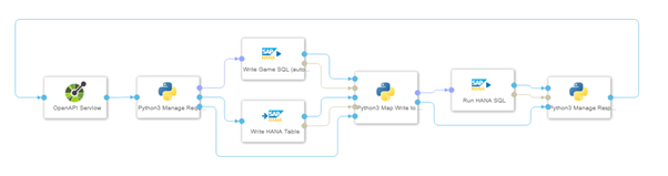
The pipeline itself contains three custom Python operators managing the data flow. Based on the operation_id included in the incoming messages, the Python operators decide how to handle the data accordingly. They have the following responsibilities:
- The first and second Python operator are responsible for passing the data to the HANA operators if necessary. If an API call does not need one of the HANA operators, the Python operator simply pipes the message through to the next Python operator.
- The second and third Python operator handle the response from the HANA operators and possible errors.
- The third Python operator consumes all messages and is responsible for sending the message that defines the response which the “OpenAPI Servelow” operator sends back as an answer to the HTTP request.
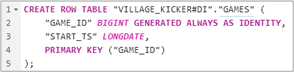
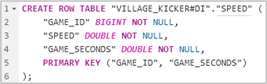
The HANA operators write or read the information which the Python operators provide to or request from them. See figure 3 for the INSERT statements of the HANA tables to which the information is persisted. In the following, we describe for each data item what the HANA operators do:
- The GAME API endpoint creates a game and returns the game information including the GAME_ID as a response. It expects an array representing the game information, which currently is only the start timestamp of the game. As the “Write HANA table” operator struggles to insert data if no key column is present, we use the “Run HANA SQL” operator for inserting the data into the HANA table. Unfortunately, the “Write HANA table” Operator does not return columns which are not passed into the operator and the “Run HANA SQL” operator returns None for an INSERT Therefore, we need to read the game with a GAME_ID of MAX(GAME_ID) in order to provide the GAME_ID in the response. With this setup, we can use it as a reference in later calls to the GOAL and SPEED APIs.
- The GOAL API endpoint creates a new goal entry from the information it receives. It expects an array including the goal information which includes the ID of the game it relates to, the ID of the team that scored the goal as well as the minute of the game and a timestamp referring to the time of the goal.
- The SPEED API endpoint persists the speed information it receives and can handle both single entries and batch data. It expects either one array including one speed entry or an array of multiple speed entry arrays at once. One speed entry array contains information about the ID of the game it relates to, the speed value of the shot and the second in which the speed value was recorded (including milliseconds in the fractional part of the float number).
Games:
Goals:
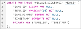
Ball speed information:
SAP Data Warehouse Cloud
Inside the SAP Data Warehouse Cloud, the project has its own space. Inside this space, a database user with read and write access is created. With this user’s credentials, SAP Data Intelligence can create a direct connection to the underlying database of SAP Data Warehouse Cloud and persist the received data there.
The data from the various tables is aggregated in several views, in order to provide relevant data to the SAP Analytics Cloud. On the one hand, there is one view each for the goals and the speed information of the current game, i.e., the game with a GAME_ID of MAX(GAME_ID). On the other hand, there is a view for the goals scored in the previous game, i.e., the game that has a GAME_ID of MAX(GAME_ID)-1.
SAP Analytics Cloud
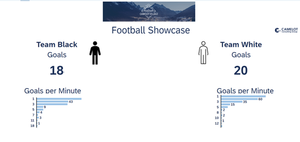
SAC is used mainly for the front-end side of the statistical dashboard creation and its connection with DWC and SAP Data Intelligence for the data transformation and display. The dashboard demonstrates both the statistical numbers on single game level as well as on the previous all played games. Total goals scored by each team were calculated in real-time via live connection as well as the goals per minute were also illustrated via bar graph as shown in the figure 8 below.
Conclusion
Overall, the project depicts the combination of tools for internal and external customer projects in a highly technical manner focusing on the connection among different systems as they work together to build a fully functional product using backend technologies such as SAP Data Intelligence to front end dashboard creation using SAP Analytics Cloud.

By loading the video, you agree to YouTube’s privacy policy.
Learn more
By the way: Playing was fun, too!