
Depending on your business sector, you may roughly catch what this title means. For the others, let’s use a French expression: “This is a Marronnier (chestnut tree),” I like this expression as it exactly describes what it is, a recurrent and non-surprising topic, like a chestnut tree blooming in spring, neither in summer nor in fall and never in winter.
The Context
Along my career I have encountered exactly the same question in each and every project: “What forecast model shall we use to forecast sporadic-demand products? The last time was just in the previous week while sharing project feedback with colleagues of my company Camelot. It is the same in all businesses, be it food, medical, spare parts, aerospace, automotive, chemicals…
And every time it leads to endless discussions between business stakeholders about which is the best algorithm that software editors like SAP or any university are pushing, emphasizing their roles in demand planning and forecasting. The results of a proposed algorithm are deeply analyzed and challenged during the project to assess the fit level of forecast modeling compared to planners’ own judgment.
Very honestly, I would remember if only one of these projects had come up with a perfect solution to forecast sporadic products. The only thing I remember is something like frustration, at best the demand planner would say “Mmm… yes, that delivers some results, which is better than nothing”.
Reasons for Failure
Let’s analyze in a bit more detail the reasons that lead to this intermediate situation that does not fully match expectations.
The proposed algorithms are either mathematical or programed. They quite struggle to interpret missing values properly, generating poor results if not worse. Good to mention that a history cleansing helps get better forecasts when running common algorithms, except… when demand is sporadic. In this case, cleansing makes the situation worse as we wipe out some of the rare data.
The business focuses on accounts, unconsciously leveraging forecasts to align them with customer dimensions. By so doing, the granularity is too detailed, generating sporadicity or at least intermittency.
Sporadic-demand products are planned together with normal continuous products. The latter often determine the time granularity that applies to all products from the solution perspective.
Disaggregation of data scares most business people, who prefer empirical methods at a granular level compared to a controlled split from an aggregated level. For instance, running a forecast at family level and disaggregating it to finished goods generates fear compared to running forecast at a finish-good level, although this is more sporadic.
If you have a different opinion, please comment!
What Should Be the Right Focus to Meet Expectations?
Whenever implementing a new solution and re-thinking process definitions, we may not be addressing the right concern properly but only extending what we are used to, the “As is”, into the future.
The right questions to ask ourselves about sporadic-demand products, are:
- Shall we really continue calculating forecasts for sporadic products with such poor results?
- Why are we so “stubborn” and “stiff” and use inappropriate or poor methods to anticipate the future for sporadic demand?
- A maxim says, “when someone has only a hammer as a tool, all problems become simple nails”. Have we got only a hammer when forecasting sporadic SKUs?
How to Address Sporadic Demand from a Supply Perspective
Thinking about how to tackle the sporadic-demand product forecast, we can consider a few other options that really address the topic and bring satisfaction. These alternatives are not only focused on demand planning. They do rely on an end-to-end thinking from demand to supply through S&OP.
1. Application of reorder points
The easiest option consists in establishing a simple ROP (Reorder Point Procedure) complemented by a smartly calculated safety stock on the planning side. An average consumption is easy to calculate and ROP therefore is straight forward. For the safety stock side, variability cannot be considered like any other material against a monthly bucketed approach, however, comparing the last three years may provide enough insight to calculate it smartly.
This option represents an inventory investment, half of the average stock and safety. Still, it is likely the case in practice, so nothing new.
From an operation management perspective, the ROP idea dramatically simplifies the replenishment process, stabilizing OTIF (on Time in Full) if not improving it. Useless to say anyone understands an ROP design without being a statistician.
In short, the ROP method, designed 80 years ago, is not an economic optimum in inventory management, however, it still brings value like simplification and protection against variability.
“Daniel! We make aircraft engines, selling them to airline companies. Prices are about 13 million Euros each at least. You advise us to keep two or three engines in the warehouse? No way!”.
Obviously, the idea going ROP has some limits, however it can be applied for most sporadic SKUs of class B and C.
A segmentation exercise on actual quantities and prices can help decide which forecast/planning method fits which SKUs.
Note: I have seen companies including all products in the company forecast in order to feed the budget figures or the sales plan. No need to incorporate sporadic SKUs in forecasting. You can easily determine a fair demand for these sporadic SKUs to be added to the budget or the sales plan, however not driving the replenishment process by means of forecast.
2. Application of advanced consumption-based planning approaches
The more advanced methods that can help manage sporadic demand are DDMRP or JIT. Obviously, these methods are not straight forward to implement, representing consistent change management and project investment. That is a subject for another article.
Usage of Advanced Statistical Methods
For the sake of a broad view on the topic, let’s come back to forecasting, performing statistical exercise on sporadic SKUs. In other words, let’s try forecasting despite granular level and sporadic time series.
If you run SAP, you may have heard about the special algorithm “Croston model” and its recent TSB evolution in IBP?
It provides average results, using a logic that is not self-explanatory.
From S4 and APO perspective, here.
Specifically for IBP, see here.
If you are not satisfied with it, or lost in complexity, you may have also searched for machine learning or whatever advanced IT algorithms to overcome the forecast quality issue with even more advanced and complex alternatives.
This logic of calling for more and more complexity happens like a headlong rush. In supply chain management, we tend to forget the end-users supposed to operate forecast.
For those organizations going for advanced methods, I would recommend creating a dedicated business analyst team, capable of mathematics and operational research, whose role would be to help operational planners to use advanced models. I have seen that happening in major companies with business excellence experts sharing their time to grow local competencies.
A Structured Alternative Method: Playing Concertina
Let’s now focus on a method that helps define an automated forecast calculation for sporadic SKUs. At the end of this exercise, either the calculated SKUs provide good results, or you need to imagine the ROP or DDMRP options.
1. The reasoning behind playing concertina
Before explaining the proposed concertina method, let’s revisit the assumptions with the statements below.
Statement 1 – Most statistical models do not work with missing values
As mentioned earlier, most of the statistical models that normal planners use follow the idea of extrapolating future values based on past values, organized in time series, by period. Most of the demand planning community frequently uses basic models like average, moving average, weighted average, first exponential smoothing. Then, planners also use more advanced models like exponential smoothing of 1st, 2nd or 3rd order, winters, or automated smoothing. Sometimes, they may use linear regression, Croston, ARIMAX or SARIMA modeling. In rare cases, planners can also use multi linear (causal) or R library to call for university models that only statisticians understand.
For most of those models, missing values bias the results. Easy example: Let’s consider a simplistic average on 12 months. Only one month has the value 120. Therefore, demand is 10 per period??? Stupid indeed from a supply chain perspective! Demand is 120 or nothing, not 10 a month. Okay, go for 120 only once, but when in the year? Look at Croston modeling to possibly help decide which month is the right one. January or September with a forecast of 120?
A more complex example: 3rd order exponential smoothing, when actuals are pretty continuous, but two or three periods are missing. Results become chaotic with an unexpected steep trend up or down, unless the planner goes fiddling with the model’s parameters, therefore being an expert.
Statement 2 – Until which level is it sporadic?
Very often, the business itself creates the problem of sporadicity. One of the reasons is that actual data gets integrated from the ERP, is aggregated (time series) by day or week, creating many empty periods.
The other regular cause is that business thinks too detailed, as involved in account management, introducing the customer dimension in forecasting.
Also seen in major MTS (Make-to-Stock) companies, in food and CPG: implementing MTO (Make-to- Order) processing when in fact, they only want to trigger the FAS (Final Assembly Schedule) on order, resulting again in introducing unnecessarily the customer dimension in forecasting.
Statement 3 – Aggregated forecasts are better than detailed forecasts.
Do I really need to comment on this statement? This is a true one! Please search ASCM publications or Google results (59 million results) or ChatGPT if you are still in doubt.
2. How to play concertina
1 – Determine the levels of continuity and variability
The base idea is to assess to which level of aggregation the sporadicity disappears, providing more continuous historical data that we know will better fulfill the statistical algorithms. To do so we need to segment data, following multiple aggregation paths to find the points of continuity. There can be many of those points. Let’s consider a few examples below.
Example 1 – The company CEO uses total revenue figures per month to anticipate next year’s turnover. No issues here unless a Covid kind of disruption occurs. The CEO can easily extrapolate the company growth, based on the past. The “continuity point” here is the company. Unfortunately, this is not an operational forecast.
Example 2 – Individual products are sporadic in the spare parts department, however aggregated by family or purchasing groups or whatever hierarchy, figures become continuous. Continuity points are one of those regrouping master data.
Example 3 – Actuals are retrieved from ERP at week level, showing sporadicity. Aggregating to month, quarter, or year usually make figures more continuous. The continuity point here is the time period.
While detecting the appropriate continuity point, it is also important to assess the volatility level of the potential aggregated figures. That will help later to determine which statistical model to use.
Note: In case of forecast automation/clustered forecast modeling, I would advise to run continuity point determination beforehand. This reduces the matrix of clusters with fewer entry columns therefore easier to finetune.
2 – Determine the appropriate forecast algorithm
Depending on the nature of the continuity point, the range of necessary forecast algorithms is drastically reduced. In other words, the forecast modeling is much easier. For instance, if you go with yearly of quarterly continuity points, no seasonality is required anymore. If you use product family/monthly periods, you may at max use 3rd exponential smoothing, which is not more complex, likely not Croston.
3 – Determine the disaggregation logic
When forecasting at aggregated level, at some point you need to disaggregate the results. This is because you later need to pass over your outputs to your supply planner colleagues, who deal with product/location only.
The disaggregation topic is largely documented on the web. There is no magic. You need to make a choice as disaggregation represents the tradeoff element of the aggregated forecast. The options are manifold:
- Disaggregation of the forecast based on actuals shifted by 12 months at detailed level
- Disaggregation of the forecast based on average of x months in the past, applied as a constant factor for all periods in the future
- Disaggregation of the forecast based on a disaggregation factor, calculated automatically and reviewed/validated manually
- Disaggregation based on a separate dummy granular forecast (automatic 3rd exponential smoothing) that represents the disaggregation factor.
- Etc…
3. Examples
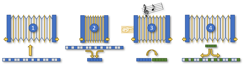
Now that the theory is given, let us imagine a couple business examples to illustrate the concept that I called the “concertina method” or the “accordion method”.
First, you extend the concertina to absorb detailed data (see figure above), second, you compress it (aggregate), third, while pulling the instrument, you play music (the simpler statistic algorithm), and finally, you finish extending it, again to deliver results back at the required detailed level by means of disaggregation logic.
Spare Parts
Although spare part management deserves a dedicated article, which I will write some time, demand is often sporadic. Depending on the business, actuals appear 1-6 times a year, in weekly buckets. Often poorly forecasted with average. Demand can gradually increase or decrease depending on the main product it is about, e.g., bearings for a special car model. Over the years, this bearing, as a spare part, will have no demand when the car model is new. When the car model is getting older, demand for the bearing increases, then the car model is decommissioned and demand for the bearing will gradually disappear. This means although this is a sporadic SKU, its demand is not just sporadic and needs anticipation, for instance, based on car model programs.
How to do? Aggregate actuals at quarterly level. If still sporadic, aggregate to yearly. Run trend model (2nd exponential smoothing), then disaggregate in a monthly or weekly bucket based on the last two years’ cumulated history.
Not to forget a safety stock calculated with last year’s variability, to ensure that distribution of the new forecast against future weeks based on last year’s sales may vary this year.
Make-to-Order
Your company produces generic products on demand. Forecasters are given the instruction to calculate the forecast at product/customer level. Results are poor to very poor. I have seen this with multibillion Euro companies.
Concertina step 2 (see figure), aggregates at product only, leaving out the customer dimension, to step 4. You should now get pretty smooth data. Now we have a weekly bucketed history showing figures everywhere. Select the appropriate forecast model to play music in step 3, this is not an issue here. Then step 4: disaggregate using a disaggregation factor combining last year‘s sales by customers, with the sales forecast for the future provided by sales representatives, and possibly with customer forecast if you are lucky.
What you get in the end is a solid forecast distributed against customers that can be now compared with any other entries such as sales forecast, customer forecast, possibly submitted to them for information.
Don’t forget that this is only a statistical forecast we are trying to refine here, therefore somewhat about 80% accuracy at best, at product/location level. Hence let’s be a little tolerant, without forgetting there are compensation processes later like S&OP, promotions, events, safety stock, and also usually expediting actions that complete the global picture. Demand planners are not alone in an empty world, responsible for delivering THE truth. Demand planning is one link in the supply chain.
Multi-Packaging and Configuration
Multi-packaging of same product, because of differentiation by language or country, or due to sales configuration that introduces many variants of the same product.
If you have a master data field that helps regrouping all similar finished products, therefore concertina step 2 is to aggregate using this field. Keep on doing as outlined in the previous paragraph.
If you don’t have such an easy field, the right product to forecast is not the finished good, but the main BOM component. See the next paragraph.
Planning a Product
You sell many variants of the same product, due to MTO, combined with language and country-specific labeling. However, what is in the pot that you sell is the same product. In this case, the product to plan is in the pot, regardless of stickers and labels. On this material you should already have a nice and smooth history made of good issue movements against production order not any sales movement, indeed. This is not a sporadic case anymore.
Conclusion
To conclude, I want to tell you a personal story about this concertina method.
It was a Proof of Value exercise that my team and I went through, to race for an IBP project implementation for a major company. The customer was providing a 36-month history for thousands of products, including customer and sales force breakdown. We had a month to grind these data and return the forecast for the next months. During this month, we spent about 3-5 days on quickly designing an IBP setup to host data. Then, we calculated the forecast, with appropriate segmentation, selectively aggregating based on previous segmentation, playing concertina to the end. We delivered the file with our forecast and ended 2nd place out of 4-5 competitors, with about 63% accuracy. I have to say I am neither a statistician nor a demand planner. I am only a reasonable consultant focused on pragmatism and simplicity, at least this is the idea.
Here, if you are a little tolerant, we can agree this result is quite good compared to the fact we had absolutely no idea about the products, no description, just a Material ID, no idea about the customers present in the history file etc… We won the project because of our position and other strengths. No doubt, with some business insights the 63% could easily grow to a satisfying level.
As a matter of fact, once we were engaged the project, forecasters and demand lead decided to forecast by product/customer/month, without any clustered forecast, business being essentially MTO. Exactly the opposite of what is said in this article, we had to play with Croston, liaise with SAP with suspicious results we could not explain etc.…
No need to say, forecast accuracy did by far not meet expectations. It was escalated to management, even to SAP, looking for new algorithms.
If you struggle with forecast quality, like the vast majority of demand planning practitioners, Camelot Management Consultants can definitely help you improve this, and you know what? This is not necessarily a lack-of-IT-capabilities issue!
Enjoying supply chain!
If you like this article, “Like” it, “Repost” it, “Comment” it, we grow by exchanging opinions!