In our previous blog posts “A short history of neural networks” and “The Unit That Makes Neural Networks Neural: Perceptrons”, we took you on a tour about how neural networks were first developed and then outlined the details of perceptrons as the basic unit of a neural net. In this blog post, we want to demonstrate how adding so-called “hidden” layers empowers neural nets to solve more complex tasks than a single-layer perceptron.
The Hidden Layer
As shown in our previous blog posts, neural networks are a class of models that are built with layers. Our last blog dealt with the simple perceptron which consists of only two layers: an input layer and an output layer. We illustrated how this simple architecture limits the perceptron to solving linearly separable classification problems only, i.e., problems that can be separated by a single straight line. Many real-world classification problems are, however, non-linear. To overcome this, the idea of the single-layer perceptron was expanded by adding more intermediate layers between the input and output layer. Those intermediate layers are referred to as “hidden” layers and the expanded network is simply called “multi-layer perceptron”.
Each node of a hidden layer performs a computation on the weighted inputs it receives to produce an output, which is then fed as an input to the next layer. This next layer might be another hidden layer or the output layer, which yields the probabilities of each label. The concept of the hidden layer gives us the power to solve complex mathematical problems, e.g., the so-called exclusive OR (XOR) problem.
Solving the XOR problem
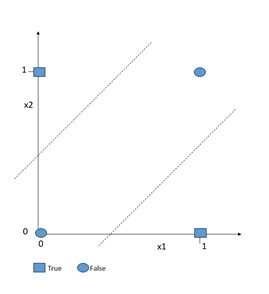
The XOR problem is the simplest problem a perceptron is not able to solve. Given two inputs, the XOR problem means that a neuron is true only if the inputs from previous neurons are not the same.
Hence, it is true given {(1,0), {0,1)}, but not for {(0,0), (1,1)}. If we depict this problem in two-dimensional space as in Figure 1, it becomes obvious that it can’t be solved with a single line, since we are not able to separate true and false data points with a single line.
However, inserting another hidden layer between the input and output layers solves the problem. We introduce a single hidden layer consisting of two neurons that are connected to each neuron of the previous input and the successive output layers, as displayed in Figure 2. Remember that each neuron has a weight and bias attached to it, which might be initialized randomly or according to some probabilistic distribution. The output at the hidden layers H1 and H2 will be calculated as follows:
- H1: σ (-x₁+x₂-0,5)
- H2: σ (x₁-x₂-0,5)
First, the weighted sum of the inputs that reach the hidden unit is calculated. Then, this sum is provided as an input to a non-linear activation function. An activation function defines how the weighted sum of the inputs is transformed into an output. In this case, we choose the sigmoid function as activation at both the hidden and output layers. The sigmoid function is an S-shaped curve that squashes any real value between 0 and 1. If the outcome of the sigmoid function is greater or equal to 0.5, we classify that node as class 1 and let the signal pass and if it is less than 0.5, we classify it as class 0 and the signal stops.
Finally, the function for the output node is as follows:
- σ (h1+h2-0,5)
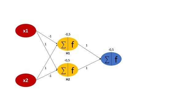 Figure 2: Adding a hidden layer to the simple perceptron
If you solve that network with all combinations of {(0,0), (0,1), (1,0), (1,1)}, you will see that the output is true for (0,1) and (1,0), but false for (0,0) and (1,1). Or in other words, the network solves the XOR problem. In this example case, the weights and biases were set in a way that the problem got solved right away. For real-world problems this is usually not the case. Here, the network needs to “learn” those parameters by repeatedly being exposed to the input data and adjusting the weights in a way to get closer to the expected output. This process of calibrating the network is called backpropagation.
Learning Hierarchical Features with Deep Networks
In the last section, we covered a neural network with a single hidden layer. Such networks are called shallow neural networks. On the other hand, any network that involves more than one hidden layer is called a deep network, which is exactly where the term deep learning stems from. Machine learning researchers or practitioners usually work with deep networks that might even consist of layers counting in the hundreds if the datasets are very large.
But what is the benefit of making neural networks deeper and deeper you might wonder? Well, deep models do something called automatic feature learning. To discriminate data into different classes, machine learning algorithms rely on features that are represented in the data and differ between classes. For example, an image classifier that classifies images into dogs and cats might use the overall size of the animal or the size and shape of the nose and other facial features.
For traditional machine learning algorithms, the data scientist is responsible for supplying those features explicitly as part of the training data along with the label information. The algorithm can then learn interactions between features and the target classes in the training phase. Deep learning models, on the other hand, do not require explicit feature information, but learn features inherently without human intervention. This can result in large amounts of time saved which would have otherwise been spent on creating features. Deep networks owe the skill of automatic feature learning to their layered topology. As Yoshua Bengio, a frontrunner in deep learning research, explains in his article “Learning Deep Architectures for AI” (2009, pdf):
“Deep learning methods aim at learning feature hierarchies with features from higher levels of the hierarchy formed by the composition of lower-level features. Automatically learning features at multiple levels of abstraction allow a system to learn complex functions mapping the input to the output directly from data, without depending completely on human-crafted features.”
Source: Yoshua Bengio, Learning Deep Architectures for AI, 2009, pdf
In case of our image classifier that could mean, in a simplified overview:
- First, the algorithm learns to detect edges appearing in the image.
- Then, basic shapes and contours.
- Then, it learns to recognize eyes, ears and other facial features,
- followed by learning to detect the face.
- And finally, combining the face with possibly other features, it can discriminate between the very abstract concepts of dogs and cats.
Hence, in a deep learning network, each layer of nodes trains on a distinct set of features based on the output from the previous layer. The further you progress within the layers, the more advanced the features your nodes can recognize, as they aggregate features learned in previous layers.
How to choose the number of hidden layers
Having introduced the rationale of the hidden layer, there is one question remaining: How many hidden layers do you include in a neural net? (See also this discussion on stackexchange)
The number of layers and the number of nodes in each hidden layer are the two main parameters that control the architecture and topology of the network. Now, if adding more layers allows for more abstract features to be learned by a network, wouldn’t it make sense to continue increasing the number of layers until we see no more significant reduction of the training error? Theoretically yes, but there are two main points to consider: First, increasing the number of layers increases computational costs as your model needs to learn more parameters. And second, when making your neutral networks deeper, the danger of overfitting gets higher. Overfitting describes when a model performs very well on the training data at hand, but its performance degrades on unseen data.
This effect occurs when the weights get adjusted in a way to “remember” the training data, but not in a way to learn the underlying feature interactions that are represented within the data. Hence, the answer is the same as in traditional machine learning: The number of layers and the number of nodes in each hidden layer are parameters that need to be tuned based on running many experiments and measuring the test error.
Drawbacks of deep learning
Given they are so powerful, you might ask why neural networks are not used for every machine learning problem. Well, they incur some drawbacks. We will discuss two of the most important drawbacks in this last section.
Resource consumption
Neural networks consume a whole lot of resources. The bigger neural networks get, the more complex they are, and hence more data and computation power are required to train them effectively.
For example, there is a famous dataset for handwritten numbers classification called “MNIST”, which consists of over 60,000 images of handwritten digits from 0 to 9. Shallow neural networks can learn and solve that problem in a reasonable time, but if you would compare that to how children learn these same ten different digits, they for sure are more efficient – they would not need to look at 60,000 images first. But neural networks are very data hungry and the deeper they get, the more data you need to feed them.
Limited explainability
Another problem is limited explainability: Since deep neural networks consist of thousands or even hundreds of thousands of neurons, it is hard to identify the one or the few neurons that were important for making a decision. This black box nature of neural networks makes their predictions hardly explainable. In business reality, however, it might be of high importance or even mandatory (e.g., for compliance) to explain why certain decisions were taken. As an example, it should be explainable why a neural network classifies debtors into “will fully repay” and “will default” in a credit scoring use case. In these scenarios, it might be a better choice to revert to machine learning algorithms that offer better transparency into how their predictions were made, like tree-based ensemble algorithms.
Find articles on related topics for Data-Driven Leaders assembled here.
We would like to thank Stefan Morgenweck und Tobias Walter for their valuable contribution to this article.