
In the previous blog post A Short History of Neural Networks we gave you a short introduction to how neural networks work and how they are modeled after our human brains. In this blog post, we will show you the most basic unit inside a Neural Network, the so-called Perceptron.
We will guide you through a lifecycle of such a Perceptron and make it clear what happens when it “works” or “predicts” and what it does when it “trains”. Finally, you will be presented with use cases and restrictions that come with these Perceptrons and learn how such a simple unit(algorithm/structure) started the first “AI Winter” which was a period where Machine Learning was considered dead.
What is a Perceptron
When Frank Rosenblatt introduced a Perceptron in 1958, it was meant to be a machine for image classification that was connected to a 20×20 pixels camera. In today’s terms, a Perceptron is just a basic algorithm that can be used for linear classification problems in Machine Learning. Binary classification means we want to predict if our input falls into one of two classes. In the example below, these two classes are 0 or 1. Another examples could be diagnosing skin cancer from images, determine if an e-mail is spam, or detection of fraudulent payment.
The four basic components of a perceptron are inputs, weights, bias and an activation function.
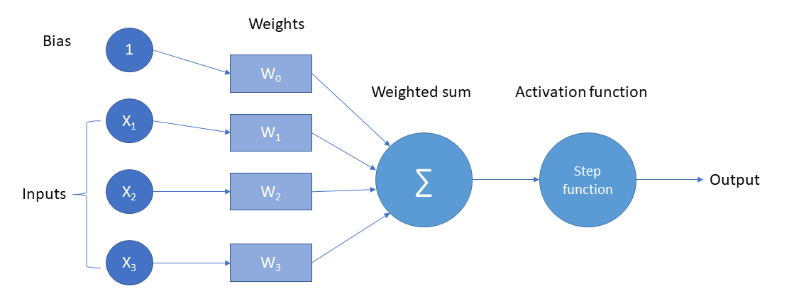
In diagram 1 you can see how a perceptron works mathematically. The input gets multiplied by the weights and then summed up until we have a single number. Theoretically, right now we have an algorithm that does regression, but since we want to use it for classification tasks,we use a so-called activation function or step function.
Let’s look at a practical example: We want to know if a master data record has all required fields filled or not. Since we only care about if the fields are filled or not, we encode this information into three binary numbers. Hence, the input we will feed into our perceptron looks like this:
<field 1 is filled>, <field 2 is filled>, <field 3 is filled>
Also for this example, let’s assume the weights for our three fields are random numbers with the values <0.2, 0.4, 0.7>. Our activation function in this case will just be a simple rounding function. If the number is greater or equal to 0.5, it will take the value 1, which means all the required fields are filled, and else it is 0, meaning that not all required fields are filled. Let’s assume our input is <1,1,0>, which means only two of the three required fields are filled. We start by multiplying our first input “1” with our first weight “0.2” and we get 0.2 as a result. If we do this for all three pairs, we receive the vector <0.2, 0.4, 0>. Now the sum of all these numbers is 0.2+0.4 = 0.6 as an intermediate result for our perceptron.
Remember that so far, we have a real number which could be useful for a regression task, but since we want to have a “yes” or “no” at the end, we apply our activation function. If we round up 0.6, we get 1 and therefore our perceptron tells us that all the required fields are filled, which is actually not the case. So what went wrong? Well, nothing really, the result was just wrong due to randomly chosen weights in the beginning.
Here comes the fun part – training! We now need to find a way to adjust the weights in a way that given our inputs, this perceptron outputs a 0 instead of a 1. Let’s do another round, but this time we set the weights to <0.2, 0.25, 0.7>. If we multiply the pairs and sum them up, we end up with
0.2*1+0.25*1+0*0.7=0.45
which is rounded down to 0 after applying our activation function. And now we can see the output is the excepted one, which means our perceptron improved. Of course, this was a very easy example since you could find the perfect weights just by looking at the numbers and finger counting. In reality, neural networks have thousands of neurons each with weights attached and possibly different activation functions, making it it impossible to just create a perfect classifier by just looking at the numbers.
Use cases and restrictions
A perceptron is a simple algorithm that can be used only for simple (binary) classification problems. However, the biggest problem with this easy algorithm is that it can only solve linear problems. If you ask yourself what linear problems are, then think about your math classes back in school where you had functions in a two-dimensional space along with axis and points. Imagine we have points that belong to the first class and points that belong to the second class in a two-dimensional space. If we can fit a line that would separate the two classes of points, then this is called a linear (classification) problem.
So why are these perceptrons not used anywhere in our complex world today? Well, they have a big drawback: They cannot solve non-linear problems, which are the type of problems we almost always face nowadays.
A glimpse on AI Winter
The perceptron and its abilities really boosted the hype about AI in the 1960s – until Minsky & Papert showed in 1969 that a Perceptron cannot solve non-linear problems and therefore won’t solve many of the problems it was supposed to solve. This was the beginning of the so-called AI winter, when fundings were stopped and AI research institutes were closed. Roughly ten years later, the idea came up that you could have layers of perceptrons that are connected to each other with non-linear activation functions which is then called a neural network. This finding as well as greatly increased computing power woke the neural networks up from hibernation.
Outlook on future blog articles
Today we showed you how a perceptron works and many perceptrons create a neural network. In our next part of the series we will demonstrate how adding additional so-called hidden layers drastically increases the complexity of problems a neural network can handle.
We would like to thank Jan Kettner and Stefan Morgenweck for their valuable contribution to this article.